Disclaimer: The notes are made from information available here and wikipedia.

Conjugate gradient is effective for solving systems of the form:

$\mathbf{A}x=b$

$x$ is an unknown vector
$\mathbf{A}$ is a known positive-definite, square, symmetric matrix
$b$ is a known vector

The CG method is most effective in solving systems where $\mathbf{A}$ is sparse. In case where $\mathbf{A}$ is dense, the solution can be found by factorizing $\mathbf{A}$ and using back substitution. On the other hand, when $\mathbf{A}$ is sparse, factorising and back-substitution become lengthy procedures.

Now, say we are finding the optimal solution of a quadratic equation $f(x)$ :

$f(x)=\frac{1}{2} x^T \mathbf{A}x-b^Tx+c$

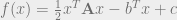
For a positive definite square symmetric matrix $A$ the equation can be solved by finding the point where the gradient of $f(x)$ becomes = 0. Therefore the solution of $f'(x)=0=Ax-b$ gives the critical point of $f(x)$ .

So why use CG?

The idea is to solve the equation not by finding the intersection of hyperplanes rather, by iterative minimization of the problem.

Method of Steepest Descent

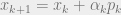
The method of steepest descent entails starting from an arbitrary point $x_0$ and consequently taking steps along the direction opposite to gradient $f'(x)$ which is $-f'(x_i)=b-Ax_i$ , to reach at the optimal point of $f(x)$ . It is convenient to say:

$x_{k+1} = x_k+ \alpha_k p_k$

Where $\alpha_k$ is the step length taken in the direction of $p_k$ which is $-f'(x)$ .

As error $e_i=x^*-x_i$ and $r_i=b-Ax_i$ $r_i$ is essentially the direction of the steepest descent i.e. $-f'(x)$ . Therefore the step length can be found by line search.

Eigenvectors and Eigenvalues

Eigenvector $v$ of matrix $\mathbf{B}$ is the non zero vector, which when multiplied with B doesn’t rotate, rather changes in length or reverses its direction. Therefore, for some scalar $\lambda$ , $\mathbf{B}v=\lambda v$ . This $\lambda$ is called the eigenvalue of vector $v$ .

Spectral radius: $\rho(\mathbf{B})=max |\lambda|$ . If the value of spectral radius is less than one, it indicates convergence. Lower the value of spectral radius, faster the convergence.

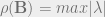
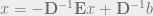
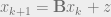
Jacobi iterative method

In pursuit of solving $\mathbf{A}x=b$ , we split $\mathbf{A}$ to matrices with its diagonal $\mathbf{D}$ and non-diagonal elements $\mathbf{E}$

$\mathbf{D}x=-\mathbf{E}x+b$
$x=-\mathbf{D}^{-1}\mathbf{E}x+\mathbf{D}^{-1}b$
$x_{k+1}=-\mathbf{D}^{-1}\mathbf{E}x_k+\mathbf{D}^{-1}b$
for, $-\mathbf{D}^{-1}\mathbf{E}=\mathbf{B}$ & $\mathbf{D}^{-1}b=z$
$x_{k+1}=\mathbf{B}x_k+z$
$x_{k+1}=\mathbf{B}(x^*+e_k)+z$ where error $e_k=x_k-x^*$
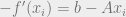
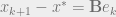
Now, at the optimal point, $x_k=x_{k+1}$ hence, $x^*=\mathbf{B}x^*+z$
$x_{k+1}-x^*=\mathbf{B}e_k$
$e_{k+1}=\mathbf{B}e_k$

Note:

Question 1: But $B$ is not the eigenvector of $x$ . How does it still converge the results?

Answer 1: Vector $x$ can be split as a sum of eigenvectors of $B$ .

$x=a*v_1+b*v_2$

$Bx=a*\lambda_1 v_1+ b*\lambda_2 v_2$

from triangle inequality,

$a*|\lambda_1 v_1|+ b*|\lambda_2 v_2| > |Bx|$

If $|\lambda_1| and |\lambda_2|$ are smaller than one, the value of LHS reduces with every increment hence converging the value of $|Bx|$

Question 2: Why split it to diagonal and non-diagonal elements?

Answer 2: a) Diagonal elements are easy to invert.

b) This is an arbitrary choice with the hope to get $B$ that has smaller spectral radius.

Now, splitting $e_k$ to respective eigenvectors of $\mathbf{B}$ ,we get corresponding eigenvalues which will eventually determine the rate of convergence of the error $e_{k+1}$ . Lesser the value of eigenvalue $\lambda_k$ faster the convergence.

Convergence

Taking a simple approach where $e_k$ is in the direction of eigenvector, $\alpha=\lambda^{-1}$ using steepest descent the optimal point is reached at one attempt.

Similarly any $e$ can be broken further into its eigenvector components. If we take all eigenvector of $\mathbf{A}$ such that their eigenvalues are same then the optimal solution is reached in one step (Spherical rather than ellipsoidal cross-section) but in case of several non equal eigenvalues, the convergence gets tough.

REVIEW

So, Steepest Descent algorithm is rougher, this is not the most efficient way while Jacobi method is smoother because every eigenvector component is reduced in every iteration.

The Method of Conjugate Directions

In case of Steepest descent method, the common problem that one runs into is going down the same vector direction again and again increasing the cost of optimisation. The best idea here would be to accumulate all these steps in the same direction to a single effective step to avoid spending more time. A convenient method to do that is using conjugate gradient method, where the search directions are A-orthogonal to each other. $e(i+1)$ is A-orthogonal to $d(i)$ :

$d(i)^T \mathbf{A}e(i+1)=0$
$d(i)^T \mathbf{A}(e(i)+ \alpha_i d(i))=0$
$\alpha_i=\frac{-d(i)^T \mathbf{A}e(i)}{d(i)^T \mathbf{A}d(i)}$
$\alpha_i=\frac{-d(i)^T r(i)}{d(i)^T \mathbf{A}d(i)}$

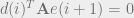
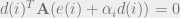
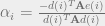
Where $d(i)$ is the search direction.

Method of Conjugate Gradient

CG is simply the method of Conjugate Directions where the search directions are constructed by conjugation of the residuals (u_i=r_i).

Conjugate gradient method